New Zealand Psychological Society conference 2019

I’ve always been a big fan of the New Zealand Psychological Society‘s annual conference.  In contrast to many conferences, it is always really welcoming and has lots of useful streams for researchers and clinicians alike.  This year I was priviliged to be able to attend with several of my fantastic PhD students and present a symposium on measurement and assessment.  A great time was had by all!

I also presented one of my favourite workshops – Silos, Gorillas, and Personality Assessment.  Slides for the symposium and workshop can be found at the links below.

Thanks NZ, you have been amazing as always!

Assessment and measurement symposium slides

Silos, Gorillas, and Personality Assessment workshop slides


Personality assessment workshops for psychologists

I will be running two group supervision workshops on personality assessment in early September, covering the NEO-PI-3 and the PAI (adolescent and adult versions).  There is a full day option in person for those in Melbourne (Saturday 7th) or two evening sessions via Zoom (Monday 2nd and 9th).  There will be a follow up consultation a month later for any questions and case discussion.  Each workshop will have no more than five participants, so it can be logged as group supervision.  The workshops are designed for provisional psychologists, but would also be useful for early career psychologists or those who want to develop their skills in personality assessment.

Why the NEO-PI-3 and PAI together?

Despite both being named “personality” measures, these are very different tools.  The NEO-PI-3 is a measure of trait personality, which is very useful for general presentations and for conceptualising difficulties experienced by individuals.  For more clinical presentations or when more complex mental illness is suspected, the PAI offers significantly more useful information for the assessing psychologist.  Being able to recognise when and how to use each type of assessment tool is a critical competency for all psychologists.

What’s included:

  • 7 hours of group supervision with a board approved supervisor
  • NEO-PI-3 and PAI for self-administration via PARiConnect online
  • Clinical case presentations
  • Guidelines for interpretation
  • Templates for reporting test data

The NEO-PI-3, PAI, and PAI-A will also be made available to participants at cost through PARiConnect between the workshop and the follow up consultation.  The total cost of the workshop, including materials and follow up consultation, is $375 per person.  Please email shane@shanecostello.net if you are interested.

About me:

I am a psychologist with endorsement in educational and developmental psychology, and a board approved supervisor.  I work in academia, private practice, and hospital settings, primarily in complex differential assessment and treatment planning roles.  I have taught personality assessment for a number of years, conducted hundreds of personality assessments in clinical and educational settings, and presented workshops on personality assessment in Australia, New Zealand, and the United States. 

ACPID 2017

It is that time of the year again!  The Australian Conference on Personality and Individual Differences is being held in Sydney, and as usual I am sitting in front of my computer late the night before the conference, working on slides.  I can only blame my low conscientiousness and organisation traits – despite my best intentions I never seem to get things done until the last minute.  If you are interested in a copy of my presentation slides, you can download them here.

The paper which I am presenting builds on an earlier conference presentation I did in 2014, and subsequently published in 2015.  This time I am looking at predicting the way people respond (not content, but their persistant pattern of responses) to personality measures, and the extent to which that pattern can be predicting using big data.  After meeting Michal Kosinski at ACPID 2016, I was inspired to try my hand at some analysis using digital behaviours, more specifically Facebook likes.  This started me on a journey to learn to use R, which is worthy of a blog post of its own.

If you want the brief findings, basically the particular pattern of responding I was interested in is acquiescence – the tendency to agree or disagree regardless of what the questions are about.  It can be predicted well from digital behaviours, but if you drill down into the actual behaviours it appears that the machine learning algorithm is picking up on subtle differences in age as a predictor of acquiescence – exactly what I found in 2015.

Shane


Calculating confidence intervals and percentiles

This post was inspired by a question posed on the Provisional Psychologists Forum Australia Facebook group.  Some cognitive ability test batteries provide interpretive information at the subtest level (eg Woodcock Johnson Tests of Cognitive Abilities – Fouth Edition; WJ-IV) while others only provide it at the higher index level (eg Wechsler Intelligence Scale for Children – Fifth Edition; WISC-5).  So while you will still get a score, such as 9 on Block Design, you won’t get the associated confidence interval and percentile rank.  The rationale for this is usually that the interpretation is more reliable at the index level and the test publisher may prefer you to only interpret at that higher level.  But the absence of such information does not mean it is not able to be calculated quite easily, providing you have a little extra information. For the first time you can use some of the stuff you learned in undergrad stats!

Here is the first equation, lets assume your Wechsler subtest score is 7:

z_score = (score – mean) / standard deviation

With Wechsler scales, the maths is pretty easy, knowing that the mean is 10 and standard deviation is 3.

z_score = (7 – 10) / 3
z_score = -1

Converting a z_score to a percentile rank can be done mathematically but there is a much easier way. Open Excel, put your new z_score in the top left cell, and in the cell to the right type in “=NORMSDIST(A1)” without the “”. This will return the percentile rank of 0.1586, or ~16th percentile.

The confidence interval is a little bit more complex but still really simple. What we are trying to account for in the confidence interval is the measurement error (or standard error of measurement, SEM), which changes depending on the subtest. Let’s assume that the reliability of our subtest was .85. Here is the next equation you need:

SEM = standard deviation x square root(1 – reliability)

SEM = 3 x square root(1 – .85)

SEM = 1.16

So now we can construct a confidence interval (CI). A 68% CI is the score +/- 1 SEM, which in this example is 5.84-8.16. A 95% CI is the score +/- 2 SEM, or 4.68-9.32. This assumes that reliability and measurement error is uniform across the range of the construct, and that the construct is normally distributed. This is often not quite the case, but it is close enough for our purposes. So in the end you can conclude that your subtest score of 7 had a 95% confidence interval ranging from 4.68 to 9.32, which is higher than 16% of the population. You can do this for any scale, as long as you have the mean, standard deviation, and reliability coefficient.


Changes in intelligence across time – meaningful or just error?

Recently there was a question posed on the Educational and Developmental Psychology Networking Australia (EDPNA) Facebook group which I found very intriguing.  A child had been assessed using the Wechsler Intelligence Scale for Children – Fouth Edition (WISC-IV; for individuals 6-16 years) approximately 10 years before, and had been reassessed using the Wechsler Adult Intelligence Scale (WAIS-IV; for individuals aged 16 and older).   We typically expect cognitive abilities to be stable across the lifespan, when comparing to similar-aged peers.  But in this case, the young person’s scores were significantly different, and there was no obvious reason for the difference.  So I started wondering if differences in ability scores across time could possibly be explained as a consequence of error rather than an actual change.

I had a quick look at the literature and didn’t find any great answers (it is a very specific question of 10 year temporal stability and correlation between types of tests after all).  So I decided to apply some statistical analysis of my own, and in doing so get to practice using R, which I have been trying to teach myself in my spare time.  For this to work, a number of assumptions have to be made – let me know what you think of these assumptions.

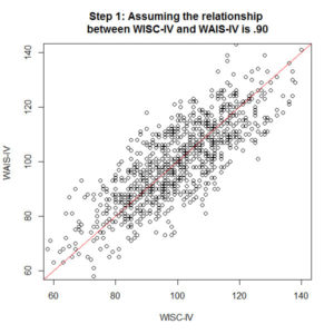
We start with simulated data (using the simulation code in SPSS discussed here) because there is no real case data available.  1000 cases are randomly generated with a whole digit score which has a mean of 100 and standard deviation of 15 (just like an index score – in fact, this is a WISC-IV index score, which one doesn’t matter).  Let’s assume that the true correlation between the WISC-IV and WAIS-IV is .90 in the population.  That’s a pretty high true correlation, maybe not realistic but good enough as a starting point.  So we generate a new score for our 1000 simulated cases which has a .90 correlation with the original score – this is our WAIS-IV index score.  In the first image at step 1, you can see this relationship plotted.

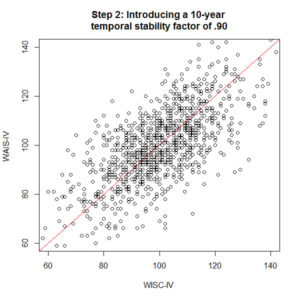
Unfortunately there is more to worry about than just the relationship between the WISC-IV and WAIS-IV.  We need to account for how stable the scores are over time, or test-retest reliability.  Let’s assume that the temporal stability of the index scores are .90 over 10 years – again a really high score, and probably very generous.  Temporal stability and the WISC/WAIS relationship errors aren’t related to each other, so we need to combine the error.  .90 relationship error multiplied by .90 temporal stability error (working in the assumption that the error is independent, and therefore compounding) gives us a new relationship between the WISC-IV and WAIS-IV across 10 years of .81.  A third index score is simulated, which correlates .81 with our original WISC-IV index score.  This is the revised WAIS-IV score after accounting for stability and relationship, and can be seen in step 2.  That graph is getting a little messy.

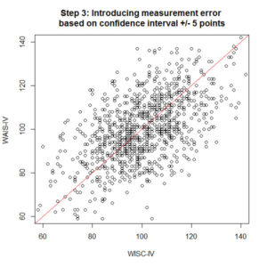
But hang on, so far we have been assuming that index scores are perfect.  A score of 100 is actually [95-105] with a 95% confidence interval (using a crude average).  The confidence interval is constructed by taking the standard error of measurement (SEM), multiplying it by two, and adding/subtracting this score to/from the index score to create a range.  If we work backwards through this calculation, the SEM is 2.5 standard score points, or 0.167 of a standard deviation.  If we take this error rate and subtract it from the “perfect” relationship a sample score would have with the population score (no measurement error), then we have a new relationship of .83 (1 – 0.167) between the achieved score and the true score.  We should take this into account in considering the relationship between our simulated index scores over time, so a new index score is generated, which is .90 relationship error multiplied by .90 temporal stability error multiplied by .83 measurement error = .56 (now our compounding error is starting to look serious).  You can see this plotted in step 3.  This step is perhaps even a little conservative, because we really only have applied the measurement error for one measurement (say the WISC-IV) and could apply it to both to be really fair.  But we are being generous at the moment.

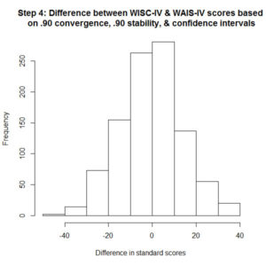
Looking at all that noise isn’t really helping to address the original question.  By how much can an index score vary over 10 years, between the WISC-IV and WAIS-IV, including measurement error?  If we take the difference between the final simulated WAIS-IV index score and the first simulated WISC-IV index score, and plot it in a histogram, we can see how large the change is for all the simulated cases.  This is shown in step 4.  Out of a sample of 1000, about 150 had WAIS-IV index scores which were 20 standard score points lower than their original WISC-IV index scores.  A further 75 simulated cases had scores 30 points lower, and about 10 cases with 40 point differences.  So about 23.5% of the sample appear to lose 20 or more standard score points (with similar numbers also showing gains).

This simulation is based on some pretty optimistic figures.  I didn’t find figures on the relationship between WISC-IV and WAIS-IV index scores (but never really tried too hard), but what if it was only .80?  And what if the 10 year temporal stability was also only .80?  Both of these scores are still really high.  A histogram modelling that shows about 26% of the sample lost 20 or more standard score points.  If the relationship was .70 for each of those parameters, about 28.5% of the sample lost that much. 

Now consider that this simulation is for only one index score.  The WISC-IV has four index scores, and even with optimistic parameters of .90, there is a 23.5% chance that each of them may demonstrate a 20 or more point loss.  Those are pretty high odds that you will find at least one index score that varies quite significantly within any individual over 10 years and between types of tools.  And this ignores any changes in typical development, incident or injury, medication, diagnosis, sleep, diet, or any other factor that you can think of which might influence a cognitive ability score. 

This is of course just a simulation study, but the mechanics of it are accurate.  If anyone finds actual parameters for 10 year test-retest stability, or the relationship between WISC-IV and WAIS-IV, we could plug them in and simulate it with 10000 cases if needed.  But it seems to indicate pretty conclusively to me that even if we are optimistic and everything relates to everything really strongly, there is still a pretty high chance of what looks like a significant change in cognitive ability scores across time could be nothing more than error.

The Krongold Outreach Program Career Assessment Service

The Krongold Outreach Program Career Assessment Service (KOP-CAS) is a program that I developed with my colleagues Zoe Morris and Nick Gamble.  Essentially, we developed a training protocol and materials for a career assessment and feedback service, which is used as a platform to develop competencies in provisional psychologists.

The intial results of the program were presented at the Society for Teaching Psychology‘s Preconference, hosted by the Society for Personality and Social Psychology‘s annual convention at San Antonio TX in January 2017.  A copy of that poster can be found here.

Over the eight months since that presentation, we have continued to develop the program.  We are excited to be presenting the latest findings at the New Zealand Psychological Society’s annual conference in Christchurch in August 2017.  A copy of the slides can be found here.

Simulating data from a correlation matrix in SPSS

Like most psychologists, my training in statistics focused on using SPSS.  It was only when I had completed my Honours research that I came to realise that there were other programs out there that might be better.  Some of those programs might even be able to do things that SPSS could not!  So I worked through AMOS, MPlus, RUMM2030, IRTPRO, and others – most only used for specific tasks rather than a true replacement.  But I always ended up back at SPSS when I could.

One of the things that I often wanted to do in SPSS was to create a simulated dataset from a correlation matrix.  Simulation studies are fascinating, and I wanted to be able to start playing with it myself.  Digging around online revealed a couple of interesting options, including simulating the active dataset.  Then I stumbled on this code, and managed to get it working!  I can’t credit where it came from, but if you are looking to simulate a dataset based on a published correlation matrix, this could help you out.

********************************************************

* Encoding: UTF-8.
*Input your desired correlation matrix and save it to a file.
*The example provided is based on four variables.
matrix data variables=v1 to v4
/contents=corr.
begin data.
1
.700 1
.490 .490 1
.408 .408 .408 1
end data.
save outfile=’C:\Users\shane\Downloads\corrmat.sav’
/keep=v1 to v4.

*Generate raw data. Change #i from 100 to your desired N.
*Change x(10) and #j from 10 to the size of your correlation matrix, if different.
new file.
input program.
loop #i=1 to 100.
vector x(4).
loop #j=1 to 4.
compute x(#j)=rv.normal(0,1).
end loop.
end case.
end loop.
end file.
end input program.
execute.

*Use the FACTOR procedure to generate principal components, which
*will be uncorrelated and have mean 0 and standard deviation 1 for each
*variable. Change “x10” to reflect a different number of variables if
*necessary, and if doing this then also change the number of factors
*(components) to generate and save.
factor var=x1 to x4
/criteria=factors(4)
/save=reg(all z).

*Use the MATRIX procedure to transform the uncorrelated variables to
*a set of correlated variables, and save these to a new file. These variables
*will be named COL1 to COL10 (or whatever is the chosen number of
*variables).
matrix.
get z /var=z1 to z4.
get r /file=’C:\Users\shane\Downloads\corrmat.sav’.
compute out=z*chol(r).
save out /outfile=’C:\Users\shane\Downloads\generated_data.sav’.
end matrix.

*Get the generated data and test correlations.
get file=’C:\Users\shane\Downloads\generated_data.sav’.

*Rename variables if desired. Replace “var1 to var10” with appropriate
*variable names.
rename variables (col1 to col4=var1 to var4).

*Test correlations.
correlations var1 to var4.

********************************************************

A quick update….

With the best of intentions, I have not been updating my blog as much as I would like……or at all if I am to be entirely honest!  But here is a quick update, as I am attending the Society for Teaching Psychology preconference tomorrow, followed by the Society for Personality and Social Psychology’s annual convention in San Antonio, Texas. Here are some of my materials for anyone who might be interested:

Slides for PeerWise presentation

PeerWise instructions document

Careers assessment poster

Ways of Thinking poster

Proper updates coming soon!

Shane

Building a blog

Building a blog from scratch has been an experience.  At this stage, I can say that I am very glad that I decided to go with WordPress.  Several years ago I built a basic HTML website for the 1st Bentleigh Scout Group (note: that link is to a much more polished website than the one I built!) and learned a little of the basics.  There is no doubt that with all of the community development and plugins available, working with WordPress is so much easier than building from scratch.

For a number of years, my wife and I owned our own business in the motorcycle apparel trade.  This was another venture into the world of website development.  I am hoping that despite my lack of coding experience, this blog will end up looking presentable.  Of course, I may end up realising that my time is better spent paying a web designer, and that I should have stuck to what I was good at!

So far, all of my social media and professional media links are up and operational; a little of my personal story is out there; my research page is under development; and my teaching page gives a little insight into what is important to me, and how well I do it.  Still to come is a “contact me” page, if I can work out how to do that without inviting an army of spammers into my inbox! 

Shane